College Football Rankings

This is a quick-and-dirty implementation Fiddler on the Proof’s Reasonable Rankings for College Football. Their proposal uses the score-differentials between games. Once you have all the scores, you solve a linear equation to rank teams based on how the did against one-another, and even consider how they did amongst similar teams.

Data

Here I gather the data for the 2024 season from https://www.sports-reference.com.

from  types import SimpleNamespace

import pandas as pd
import duckdb
import numpy as np

import requests
from bs4 import BeautifulSoup

import matplotlib.pyplot as plt
import seaborn as sns
import plotnine as pn

url = "https://www.sports-reference.com/cfb/years/2024-schedule.html#schedule"

response = requests.get(url)

soup = BeautifulSoup(response.content)

# Find the table (inspect the webpage to find the correct table tag and attributes)
table = soup.find("table", id="schedule")

# use these table headers
headers = [
    "week",
    "date",
    "time",
    "day",
    "winner",
    "winner_points",
    "home",
    "loser",
    "loser_points",
    "notes"
]

# Extract table rows
rows = []
for tr in table.find("tbody").find_all("tr"):
    row = []
    for td in tr.find_all("td"):
        row.append(td.text)
    rows.append(row)

# Create pandas DataFrame
scores_raw = (
    pd.DataFrame(rows, columns=headers)
    .dropna(subset=["week"])
)
scores_raw.iloc[0]

week                              1
date                   Aug 24, 2024
time                       12:00 PM
day                             Sat
winner                 Georgia Tech
winner_points                    24
home                              N
loser            (10) Florida State
loser_points                     21
notes                              
Name: 0, dtype: object

Here I clean up the scores table.

scores = duckdb.query("""
with scores as (
  select
    row_number() over() as game_id
    , trim(regexp_replace(winner, '(\(\d+\))', '')) as winner
    , trim(regexp_replace(loser, '(\(\d+\))', '')) as loser
    , cast(coalesce(nullif(winner_points, ''), '0') as int) as winner_points
    , cast(coalesce(nullif(loser_points, ''), '0') as int) as loser_points
  from scores_raw
  where 1=1 and week is not null
)
select
  *
  , loser_points
  , winner_points - loser_points as diff_points
from scores
where 1=1 
    and winner_points + loser_points > 0
""")

duckdb.query("select * from scores limit 4")

<>:1: SyntaxWarning: invalid escape sequence '\('
<>:1: SyntaxWarning: invalid escape sequence '\('
/var/folders/bm/vmrvtfpd56v9sw0pb7c_rp0w0000gp/T/ipykernel_37883/3745766914.py:1: SyntaxWarning: invalid escape sequence '\('

┌─────────┬────────────────────┬────────────────┬───────────────┬──────────────┬────────────────┬─────────────┐
│ game_id │       winner       │     loser      │ winner_points │ loser_points │ loser_points_1 │ diff_points │
│  int64  │      varchar       │    varchar     │     int32     │    int32     │     int32      │    int32    │
├─────────┼────────────────────┼────────────────┼───────────────┼──────────────┼────────────────┼─────────────┤
│       1 │ Georgia Tech       │ Florida State  │            24 │           21 │             21 │           3 │
│       2 │ Montana State      │ New Mexico     │            35 │           31 │             31 │           4 │
│       3 │ Southern Methodist │ Nevada         │            29 │           24 │             24 │           5 │
│       4 │ Hawaii             │ Delaware State │            35 │           14 │             14 │          21 │
└─────────┴────────────────────┴────────────────┴───────────────┴──────────────┴────────────────┴─────────────┘

Construct the “game matrix,” which is made up of -1,0,1.

• Each row represents a game
• Each column represents a team
• An entry is 1 if the team won that game, -1 if it lost that game, 0 otherwise

Each game will have a corresponding score, which we keep in another vector.

teams = duckdb.query("""
with teams as (
  select distinct winner as team
  from scores
  union all
  select distinct loser as team
  from scores
)
select team
from teams
order by team
""")

team_mapping = {team: i for i, team in enumerate(teams.to_df()['team']) }

game_matrix = np.zeros((scores.shape[0], teams.shape[0]))
for i, row in scores.to_df().iterrows():
  game_matrix[i, team_mapping[row['winner']]] = 1
  game_matrix[i, team_mapping[row['loser']]] = -1

"{} games, {} teams".format(*game_matrix.shape)

'919 games, 367 teams'

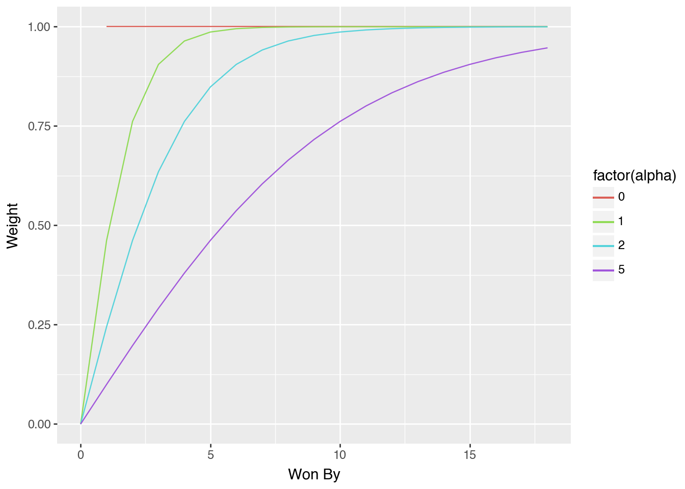
What’s a game worth?

The Fiddler maps a score-differential to a weight between 0 and 1. They recommend the function below. It accepts the number of points the winners won by (i.e. a positive number) and returns a weight between 0 and 1 (1 is better than 0).

def weigh(points_won_by, alpha:float=1.0):
  return (2 / (1+np.exp(-points_won_by / alpha))) - 1

There has a tunable parameter, alpha, which means we can decide how to weigh different wins, e.g. - when alpha=0, “a win is a win,” so a team that wins by 1 point is just as good as a team that wins by 14 points - when alpha=5, a team that wins by 1 point doesn’t get a strong weight (closer to 0), while a team that wins by 14 points gets a weight of ~0.8.

As alpha increases, teams need larger point differentials to do well.

(
  pd.concat([(
      pd.DataFrame({"Won By": np.arange(0, 19)})
      .assign(alpha=a)
      .assign(Weight=lambda df: weigh(df["Won By"], alpha=a))
    ) for a in [0, 1, 2, 5]
  ], ignore_index=True)
  .pipe(pn.ggplot)
    + pn.geom_line(pn.aes(x="Won By", y="Weight", color="factor(alpha)"))
)

/Users/pj/Documents/trainorpj.github.io/.venv/lib/python3.13/site-packages/plotnine/geoms/geom_path.py:100: PlotnineWarning: geom_path: Removed 1 rows containing missing values.

So what alpha should we choose? I would work backwards from a score, e.g. “a 14-point (2 touchdowns) win is a decisive win.”

Below I’ve plotted the distribution of points the winner won by. We see that 14 points is the median, so my reasoning feels decent.

(
  # point diff ecdf
  scores.to_df()
  .pipe(lambda df: (
    pn.ggplot(scores.to_df())
    + pn.stat_ecdf(pn.aes("diff_points"))
    # plot median
    + pn.geom_label(x=df.diff_points.median(),y=0.5,label=df.diff_points.median())
    + pn.labs(title="Point Differential ECDF")
  ))
)

Using our eyeballs to compare the two plots above, alpha=2 is a reasonable parameter, since it counts 14-point games as a “decisive” victory.

Ranking the Teams

With this we can set up a linear equation:

games_matrix * team_weights = game_weights
^known^^^^^^   ^unknown^^^^   ^known^^^^^^        

At this point I like to test my assumptions about the shapes and content of my data:

num_games = scores.shape[0]
num_teams = teams.shape[0]

assert game_matrix.shape == (num_games, num_teams)
assert (game_matrix==1).sum() == num_games # winners get a 1
assert (game_matrix==-1).sum() == num_games # losers get a -1

example_game_weights = weigh(scores.to_df().diff_points, 2)
assert example_game_weights.shape == (num_games,)
assert ((example_game_weights>=0) & (example_game_weights<=1)).sum() == num_games # values between 0 and 1

"No errors!"

'No errors!'

Now we can solve this equation. Once we have team_weights, we can pull the top 12 to get our finalists.

def solve_for_team_weights(games_, teams_, diff_points_, alpha=2):
  weights = weigh(diff_points_, alpha=alpha)
  pseudoinverse = np.linalg.pinv(games_)
  rankings = pseudoinverse @ np.array(weights)

  return pd.Series({
      team: rankings[i]
      for i, team in enumerate(teams_.to_df()['team'])
  })

rankings = solve_for_team_weights(
  game_matrix, 
  teams,
  scores.to_df().diff_points
)

# get top 12
rankings.sort_values(ascending=False).head(12)

Ohio State        1.665191
Oregon            1.548168
Notre Dame        1.468274
Penn State        1.333366
Texas             1.324272
Indiana           1.217931
Georgia           1.100962
Illinois          1.087538
South Carolina    1.084789
Mississippi       1.081674
Brigham Young     1.078441
Michigan          1.046878
dtype: float64

Sensitivity

I’m curious how changing alpha changes the top-12 composition. Recall that increasing alpha means we weigh bigger score differentials more heavily.

As we increase alpha, we see that:

• Ohio State is always #1
• Alabama makes it for alpha>2
• The higher (i.e. worse) seeds are slightly more competitive
• Miami gets in at alpha~=12

sens = SimpleNamespace()
sens.data = []
sens.fig, sens.ax = plt.subplots()

for a in np.linspace(0, 20, 11):
  sens.tw = (
    solve_for_team_weights(
      game_matrix,
      teams,
      scores.to_df().diff_points,
      alpha=a
    )
    .sort_values(ascending=False)
    .head(12)
    # I don't like pandas
    .reset_index().rename(columns={"index": "team", 0: "team_score"})
    .assign(alpha=np.round(a), seed=lambda df: df.index+1)
  )
  sens.data.append(sens.tw)

(
  pd.concat(sens.data, ignore_index=True)
  .pivot(index="team", columns="alpha", values="seed")
  # sort by avg rank
  .pipe(lambda df: df.loc[df.max(axis=1).sort_values().index])
  .pipe(lambda df: sns.heatmap(df, annot=True, ax=sens.ax))
)

<Axes: xlabel='alpha', ylabel='team'>